Arctic Sea Ice Reaches 2026 Annual Minimum Extent

Daily images of ice cover in the Arctic Ocean show sea ice melting around the pole from March 15, 2026 to Sept. 12, 2026.
Trent Schindler/NASA’s Scientific Visualization Studio

Arctic sea ice reached its annual minimum extent on Sept. 12, according to NASA and the National Snow and Ice Data Center (NSIDC) at the University of Colorado Boulder. The ice covered an estimated 1.78 million square miles (4.6 million square kilometers), tying 2008, 2010, and 2025 for the 10th-lowest minimum in the satellite record.

The 2026 minimum is consistent with patterns observed in the satellite record. The past 20 years, from 2007 through 2026, have produced the 20 lowest annual Arctic sea ice minimum extents observed since continuous satellite measurements began in late 1978.

Arctic sea ice grows during the dark, cold autumn and winter and retreats as temperatures rise during spring and summer, typically reaching its lowest extent in September. Weather conditions can cause substantial differences in the amount of ice that melts from one summer to another.

Over the last decade, for example, increased cloud cover has prevented solar radiation from further accelerating the melt of sea ice, according to Linette Boisvert, a sea ice scientist at NASA’s Goddard Space Flight Center in Greenbelt, Maryland.

That has contributed to relatively stable September sea ice extent in recent years. “We’ve plateaued, but we’re still low relative to the earlier part of the record,” said Walt Meier, a senior research scientist at NSIDC.

Antarctic sea ice extent approaches annual maximum

At the opposite end of the planet, Antarctic sea ice is approaching its annual maximum following a fluctuation during August.

Sea ice around Antarctica declined by roughly 116,000 square miles (300,000 square kilometers) over a six-day period before resuming its seasonal growth. Meier said the decline appeared to be associated with weather conditions that pushed and compacted the thin, mobile ice near its outer edge.

“Those types of things happen all the time,” Meier said. “But the magnitude of it certainly is unusual.”

Antarctic sea ice varies more from year to year than Arctic sea ice because, in contrast to the Arctic, it is not surrounded by land and can respond more freely to changing wind and weather conditions. But Antarctic sea ice extent at its annual maximum has generally been lower in recent years. Because of this large year-to-year variability, Boisvert and Meier remain cautious about characterizing the change as a long-term trend.

Scientists have tracked polar sea ice from space for nearly five decades. During that time, NASA and the National Oceanic and Atmospheric Administration (NOAA) used a series of satellite instruments to maintain a continuous sea ice record, beginning with NASA’s Nimbus-7 satellite, which began observations in October 1978. The record continued with instruments aboard Defense Meteorological Satellite Program satellites beginning in 1987 and NASA’s Aqua satellite from 2002 to 2011. Today, scientists continue the record using data from the Advanced Microwave Scanning Radiometer 2 (AMSR2), launched in 2012 aboard JAXA’s (Japan Aerospace Exploration Agency) GCOM-W satellite.

Antarctic sea ice typically reaches its annual maximum in late September or early October. NASA and NSIDC will announce the 2026 maximum after scientists confirm that seasonal ice growth has ended.

Media contact: Elizabeth Vlock
NASA Headquarters

Source: science.nasa.gov

Curiosity Blog, Sols 5010-5015: Checking out the Bands

3 min read

Curiosity Blog, Sols 5010-5015: Checking out the Bands

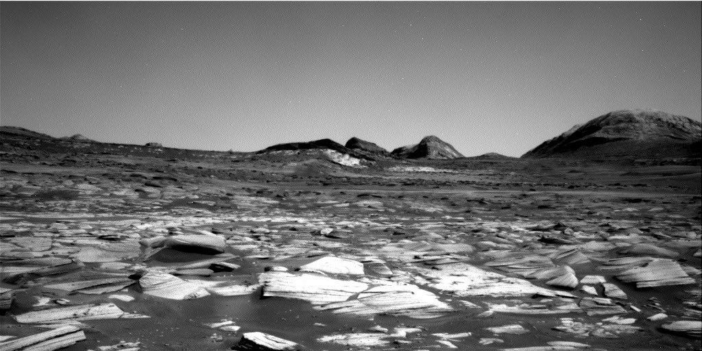
A grayscale image of the Martian surface taken by the Curiosity rover. The immediate foreground features a dense field of jagged, light-colored, thinly-layered rock fragments resting on a bed of darker sand or dust. The barren terrain gently slopes upward toward the horizon, where a cluster of dark, rugged hills and a larger, rounded mountain peak on the far right stand out against a smooth, featureless sky.
NASA’s Mars rover Curiosity acquired this image, showing the path ahead. The subtle banding can be picked out here in tonal differences. Curiosity captured the image using its Right Navigation Camera on Sept. 14, 2026 — Sol 5014, or Martian day 5,014 of the Mars Science Laboratory mission — at 02:05:20 UTC.
NASA/JPL-Caltech

Catherine O’Connell-Cooper, APXS Strategic Planner and Payload Uplink/Downlink Lead, University New Brunswick, NB, Canada

Earth planning date: Friday, Sept. 11, 2026

This week we had two planning days (Tuesday and Friday), as Monday was Labor Day in North America, where many of the Curiosity team are based. Labor Day (the first Monday in September) marks the end of summer holidays and thrills, and the return to more typical routines and back to school.

The MSL team has marked several important milestones within the past few weeks — marking our 14th “Landiversary” on Aug. 6 and surpassing the 1-kilometer elevation mark and our 5000th sol (Martian day) in early September. Our next big date is not until Nov. 26, the 15th anniversary of launch, and so it feels like Curiosity is also back to a more routine schedule at this point.

We are moving up the valley known informally as “Valle Grande.” In recent weeks, we climbed up over what we interpreted as an “erosional supersurface” (which marks a gap in the usual rock record) and are now traversing through a subtly banded area. Bands are 25-200 meters (about 80-650 feet) in diameter, with morphological changes, such as bands with more sand and less rocky outcrops (which often appear darker from a distance because there is more sand) and others where outcrops seem more continuous that allow us to mark out rough contacts between them.  

The terrain this week was characterized by sparse outcrops with a rough texture, often nodular, surrounded by lots of sand and coarse pebbly sand. On Tuesday APXS and MAHLI investigated brushed nodular bedrock at “Cerro Armazones” and “Monte Melimoyu.” ChemCam acquired LIBS on a knot of dark-toned nodules at “Tuta Huallpas” and the dark-toned float rock “Acllahuasi.”

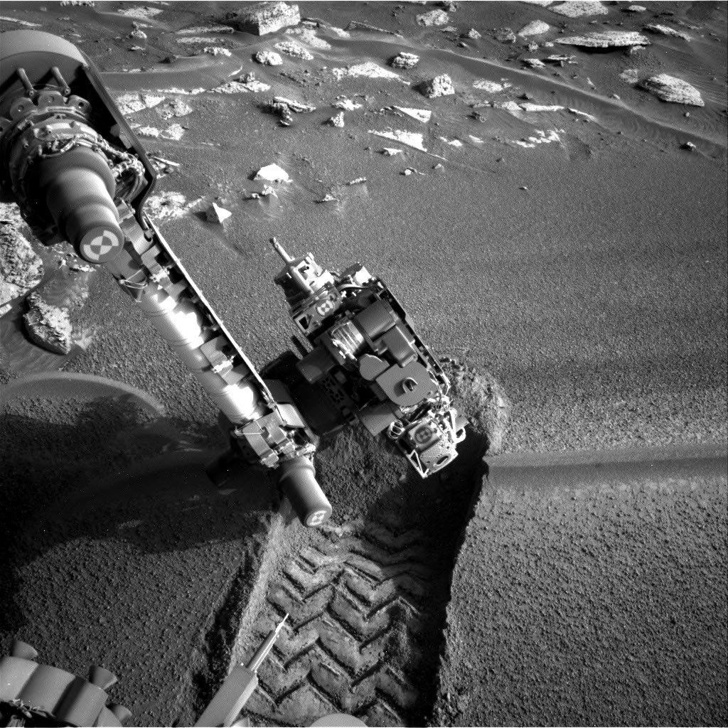
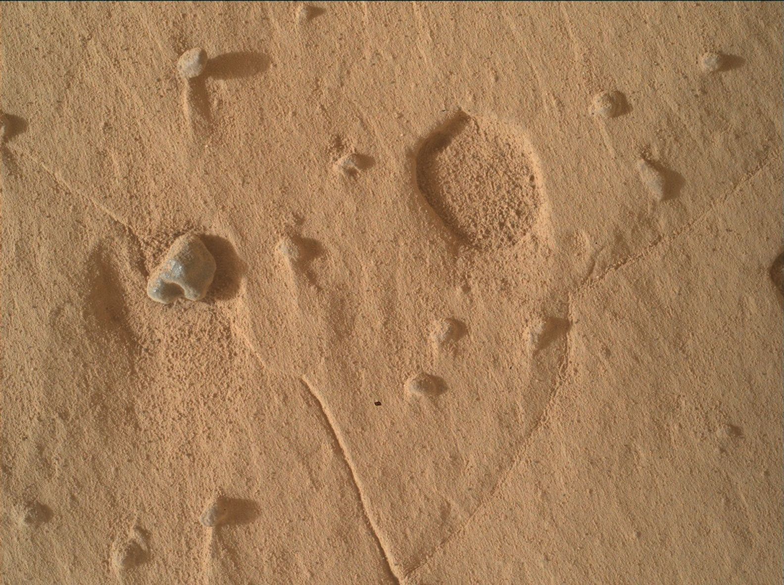
On Friday, after a drive of about 60 meters (nearly 200 feet), we found ourselves with mostly sand close to the rover and just one small rough-textured outcrop close enough for contact science and LIBS. Fortunately, the block was extremely interesting, with abundant small flakes and chips incorporated and laminated areas that are a bit smoother. We will investigate the rougher textures with MAHLI (“Yungay” and “Chiu Chiu”), APXS (Chiu Chiu) and ChemCam LIBS (“Puya Raimondii”) and a smoother area with LIBS (“Liolaemus Tacnae”).

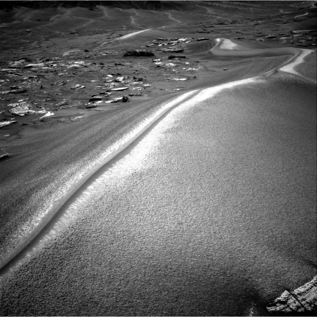
Across both plans, the ChemCam long-distance imager and camera teams were hard at work. In addition to near-field images, which focus on areas close to the rover, both Mastcam and ChemCam acquired several larger mosaics on the buttes on either side of us (“Mishe Mokwa” and “Cordillera”) and looking back to the small butte “La Linea.” Mastcam also took some mosaics documenting the “Chocolatal” scuff, which we analyzed last week, and a larger mosaic of the “Sullivan Field” sand field where Chocolatal is located. Sullivan Field contains sand ripples, mega ripples, and transverse aeolian ridges, and was named by the team in honor of the late Robert Sullivan, a world expert on Martian sands and cherished member of the Curiosity science team.

In parallel to all the geology activities, the environmental team planned their usual full schedule of monitoring activities, such as dust-devil movies, suprahorizon movies looking at the crater rim, and tau images, which look at dust in the atmosphere.

Navcam and Mastcam acquired images of the path ahead in our drive direction. The subtle bands can just about be picked out here, by looking at tonal differences. It will be very interesting to see how these look and vary from each other when we get close enough to each one.

A rover sits on the hilly, orange Martian surface beneath a flat grey sky, surrounded by chunks of rock.
NASA’s Curiosity rover at the base of Mount Sharp
NASA/JPL-Caltech/MSSS

Details

Last Updated

Sep 22, 2026

Related Terms

Source: science.nasa.gov

NASA Aircraft to Make Low-Altitude Research Flights Over Colorado

A two-engine aircraft sitting in front of a hangar.
A photo of the Dynamic Aviation A200 aircraft, which will conduct low-flying research flights over farmland near Greeley, Colorado, to measure emissions in October 2026.
Dynamic Aviation

Agricultural emissions represent an important and understudied part of Earth’s land and atmosphere systems. The FarmFlux mission will deploy more than a dozen sensors to measure ozone, methane, ammonia, particulates, and other pollutants rising from agricultural lands and animal farms and the interaction with the Earth’s atmosphere. The mission is jointly led by NASA’s Goddard Space Flight Center in Greenbelt, Maryland; Colorado State University; and Boston University. 

The Colorado deployment is the first series of flights for the FarmFlux mission. Additional low-altitude research flights are scheduled over farmland in Amarillo, Texas, from late October to early November. For the March to July 2027 growing season, research flights with a NASA P-3 Orion aircraft are scheduled in the Midwest and California’s Central Valley with a focus on croplands. 

For more information about the FarmFlux mission, visit:

https://espo.nasa.gov/farmflux

By Sharon Teitelbaum

NASA’s Ames Research Center in California’s Silicon Valley

Source: www.nasa.gov

NASA’s Hubble Telescope Reaches Milestone, Looks for Elusive Supernova

Several galaxies shine against black space, with a large cluster near center-left.
An image from NASA’s Hubble Space Telescope of galaxy cluster MACS J0417 is part of repeated observations to monitor for the reappearance of supernova Athena, which can help astronomers measure the expansion rate of the universe.
NASA, ESA, STScI, M. Pascale (UCLA); Image Processing: J. DePasquale (STScI)

NASA’s Hubble Space Telescope captured this image of massive galaxy cluster MACS J0417 (left of center) on Sept. 19, 2026. This galaxy cluster acts as a gravitational lens, bending and magnifying light from objects far behind it. Supernova Athena, discovered by NASA’s James Webb Space Telescope in 2025, is predicted to reappear between now and early March 2027. Measuring the timing of Athena’s reappearances can help researchers map the mass of MACS J0417, which acts as a magnifying, foreground lens for distant objects, and refine our understanding of the expansion rate of the universe.

Hubble also completed its 200,000th orbit around Earth on Sept. 19, marking another new milestone for an observatory that continues to transform our understanding of the universe.

Read more about Hubble and this recent milestone.

Image credit: NASA, ESA, STScI, M. Pascale (UCLA); Image Processing: J. DePasquale (STScI)

Source: www.nasa.gov

Risk of Hydrazine Use Following Freeze–Thaw Exposure

For more information, contact Jonathan E. Jones, Langley Research Center, [email protected]

Download the PDF version

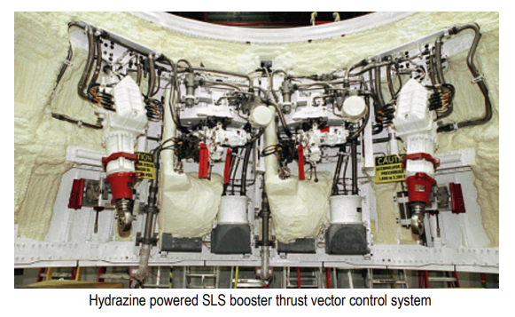
The purpose of this Technical Bulletin is to communicate the risks associated with freeze–thaw cycles in hydrazine monopropellant systems and to provide general recommendations for mitigating damage, operational hazards, and loss of system reliability in propulsion and auxiliary hydrazine systems.

Background
Hydrazine (N2H4) freezes near 1.6°C, and its phase transition is known to introduce risks to flight hardware. Multiple NASA programs have historically encountered hydrazine freeze related issues:

• Space Shuttle APU hydrazine lines were vulnerable to freeze induced contraction followed by thaw induced over expansion, capable of bursting plumbing. Shuttle flight rules permitted no more than two freeze–thaw cycles before considering the system degraded or failed.1

• Voyager propulsion systems faced mission threatening scenarios as hydrazine temperatures approached the freezing/slush formation range (0.1–1.6°C). Detailed thermal modeling was required to prevent freezing of lines, blockage, and thruster malfunction.2

• Hydrazine thermodynamic properties confirm significant changes in density and pressure across phase transitions, emphasizing the sensitivity of propellant lines to freeze–thaw stress.3

These combined lessons form the basis for risk identification and mitigation.

Problem Summary
Freeze–thaw exposure of hydrazine systems presents the following critical risks:

• Structural Damage Hydrazine contraction during freezing allows additional propellant into confined lines, producing “superpacked” conditions that cause line or fitting rupture upon thaw.2

• Valve, Seal, and Diaphragm Compromise Elastomeric components and precision valve seats may experience cracking, distortion, or loss of sealing capability due to differential thermal expansion. Voyager thermal assessments highlighted susceptibility of long stainless steel runs to asymmetric temperature profiles.2

• Line Blockage and Slush Formation Partially thawed hydrazine can remain “slushy,” restricting flow, altering mass flow rates, and causing thruster hard starts or misfires.2

• Hazardous Leaks Freeze induced damage may allow hydrazine to escape confinement, posing significant toxicity, reactivity, and ground crew exposure hazards.

• Loss of System Reliability As documented in Shuttle operations, hydrazine systems exposed to freeze–thaw cycles become life limited, reducing redundancy and mission availability.1

• Thermal Margin Uncertainty Voyager experience demonstrated that simple temperature readings cannot reliably determine true line temperature, necessitating high fidelity thermal modeling.2

Recommendations Prevention Measures
• Maintain Hydrazine Above Freezing Margin Keep all hydrazine systems above freezing, using heaters, insulation, blankets, or warm gas purge. Include uncertainty analysis in modeling and testing to ensure appropriate margins against freezing are maintained during all phases of operation.

• Avoid Uncontrolled Cooling During Ground Operations Ensure that tank, line, and valve components remain in environmentally controlled areas until integrated into the vehicle.

Post Freeze Response Protocol
If freezing cannot be ruled out:

• Suspend System Use Do not operate the hydrazine system until engineering evaluation is completed.

• Assess Number of Freeze–Thaw Cycles Treat each cycle as life limiting, an engineering assessment (static and fatigue) should be conducted based on conservative estimates of the line pressures during/after freeze/thaw cycles to understand potential line/component damage. Appropriate margin should be applied based on analysis uncertainty and/or underlying assumptions.

• Conduct Integrity Verification Perform pressure decay tests, NDE (if design allows), and valve health assessments.

• Implement Slow, Uniform Thawing To prevent thaw induced over pressure, warm hardware gradually and evenly. Shuttle experience with “superpacking” reinforces the necessity of controlled thawing.

Thruster and Valve Operational Readiness
• Ensure catalyst beds and valves reach proper thermal operating conditions before commanding any flow.

• Conduct pre start thermal stabilization periods, especially when flight readiness temperatures are marginal.

Thermal Modeling and Monitoring
• Utilize high fidelity thermal line modeling, emulating Voyager’s detailed propellant line modeling approach.2

• Avoid relying solely on bulk plate or tank temperatures to infer line readiness.

• Use thermal analysis and test to guide instrumentation placement on of the flight systems to monitor key temperatures set points.

Documentation and Incident Tracking
• Record all freeze exposures as reportable anomalies.

•Assign engineering disposition and track hardware life reduction accordingly.

Conclusion
Hydrazine freeze–thaw cycles present significant structural, operational, and safety risks for propulsion and auxiliary systems. Historical NASA programs show that prevention of hydrazine freezing is the most effective mitigation, with freeze exposure requiring formal engineering assessment, life limit adjustments, and controlled recovery procedures. Adhering to these recommendations will reduce risk to personnel, flight hardware, and mission success.

References
1. Space Shuttle Operational Flight Rules, Vol. A. All Flights, Mission Operations Diretorate, 20 June 2002. 2. W. C. Ledeboer, “Creating a Voyager Thermal Model 39 Years Into the Flight Mission, Along With Model Correlation and Application,” 8 July 2018. 3. J. L. Haws and B. G. Harden, “Thermodynamic Properties of Hydrazine,” Nov 1965.

Source: www.nasa.gov

An Epic View of the Seasons

Four full-disk images of Earth are arranged in a two-by-two grid. The December image on the upper left shows the South America centered with Antarctica visible. The June image features parts of North America and Arctic sea ice that were not visible in December. The March and September images have South America and North America in more intermediate positions.
Images from NASA’s EPIC (Earth Polychromatic Imaging Camera) aboard the NOAA mission DSCOVR (Deep Space Climate Observatory) show Earth on the December and June solstices and the March and September equinoxes, illustrating how the tilt of Earth’s axis shifts the continent’s apparent positions through the year.
NASA Earth Observatory/Michala Garrison

Most kids learn in elementary school that the seasons are caused by Earth rotating on a tilted axis during its yearly orbit around the Sun. The substantial tilt, about 23.5 degrees, is thought to be the result of an ancient planetary body, Theia, smashing into Earth about 4.5 billion years ago, in the same cataclysmic collision that formed the Moon.

To visualize why Earth has seasons, imagine the planet as a spinning top tilted to one side. Around the June solstice, the Northern Hemisphere leans toward the Sun, bringing more direct sunlight and longer days. Around the December solstice, the Southern Hemisphere does the same. That’s why June ushers in summer and warm weather in the Northern Hemisphere, while December does so in the Southern Hemisphere.

The March and September equinoxes serve as the midpoints between these two seasonal extremes. On those days, the terminator—the boundary between the sunlit and dark sides of Earth—runs directly through both poles. As a result, the Northern and Southern Hemispheres receive almost the same amount of sunlight, and day and night are nearly equal in length.

What do the seasons look like from about one million miles away? That’s the view provided by NASA’s EPIC (Earth Polychromatic Imaging Camera) aboard the NOAA mission DSCOVR (Deep Space Climate Observatory). By maintaining an orbit that puts the spacecraft between the Sun and Earth roughly 1.6 million kilometers (1 million miles) from Earth, the camera has a nearly continuous view of the sunlit hemisphere. As Earth spins during the course of a day, EPIC captures a full-disk image of the planet’s sunlit face every few hours.

The four images above, taken at roughly the same time of day, show how EPIC’s view of the Western Hemisphere changes over the year, from the December solstice (upper left) to the March equinox (upper right), June solstice (lower left), and September equinox (lower right). The most striking difference is between the two solstices. In December, South America lies near the center of the disk and much of Antarctica is visible, while North America is partially out of view. In June, Earth’s tilt means the situation is reversed: the Northern Hemisphere and North America are more centered, Arctic sea ice comes into view, South America is offset, and Antarctica is completely out of view.

There are other notable differences among the four images. Earth looks slightly smaller during the March and September equinoxes, for instance. That’s because DSCOVR was tens of thousands of miles farther away from Earth on those dates than on the solstices. On December 21, 2023, DSCOVR was 1,447,327 kilometers (899,327 miles) from Earth compared with 1,561,901 kilometers (970,520 miles) on September 22, 2024.

The slight difference in Earth’s apparent size has nothing to do with Earth’s tilt. Instead, it occurs because DSCOVR follows a looping, three-dimensional path called a Lissajous orbit to keep the spacecraft near Lagrange point 1, where the combined gravitational pull of the Sun and Earth and the centrifugal pull of the satellite balance out, making it easier for engineers to maintain the spacecraft’s position without using much fuel. DSCOVR’s distance from Earth swings between its maximum and minimum roughly every three months, and the timing drifts throughout the year because of lunar influences and orbital maneuvers. In 2024, the orbit happened to put the spacecraft slightly farther from Earth at both equinoxes, but that is not always the case.

There’s one other notable way the images differ. Because of DSCOVR’s Lissajous orbit, the angle between the Sun, Earth, and satellite varies between 2 and 12 degrees, explained Alexander Marshak, the deputy project scientist for the DSCOVR mission. Earth appears as a fully illuminated disk at smaller angles and less rounded at larger angles, like a “bite” has been taken out, similar to a gibbous phase of the Moon. For this set of images, the September 22 image has a slightly lower angle (8.1°) than the December 21 image (10.3°), making it appear slightly rounder and fuller. The angle between the Sun, Earth, and satellite in the other two images is between 9° and 10°.

“You can see the subtle influence of the changing orbital geometry in these images,” Marshak said. “But the most obvious changes—the apparent location of the continents—are due to Earth’s tilt.”

EPIC’s vantage point offers a perspective that makes it easier to understand and visualize why Earth has seasons, but after more than a decade in space, the mission has also opened up new approaches to understanding and observing how daily and seasonal cycles play out on a planetary scale. It has collected more than a decade of diurnal and seasonal data on many key features on Earth, including vegetation, clouds, ice, snow, UV radiation, ocean color, and aerosols.

NASA Earth Observatory image by Michala Garrison, using data from DSCOVR EPIC. Story by Adam Voiland.

References & Resources

You may also be interested in:

Stay up-to-date with the latest content from NASA as we explore the universe and discover more about our home planet.

A Moonlit Earth as Seen From Artemis II

4 min read

An astronaut’s photo, taken en route to the Moon, reveals our planet and its place in space in a novel…

Article

June 2026 Satellite Puzzler

2 min read

Your challenge is to tell us the location of the satellite image and why it is interesting.

Article

Great Balls of Fire

4 min read

An astronaut on the International Space Station was surprised to photograph a shower of light streaking through the darkness while…

Article

Source: science.nasa.gov

NASA’s Chandra Finds Unusual Objects in Pinwheel Galaxy

Researchers found 84 so-called hypersoft X-ray sources in M101, Messier 31, and four elliptical galaxies. This newly-discovered class of objects give off very low-energy X-rays and likely high levels of ultraviolet light. Their existence may help explain questions around Type Ia supernova explosions and the intergalactic medium. These images of the face-on spiral galaxy M101 show X-ray data from Chandra and an optical image from the Hubble Space Telescope.
X-ray: NASA/CXC/Univ. of Alabama/M. Muhibullah et al.; Optical: NASA/ESA/STScI; Image Processing: NASA/CXC/SAO/N. Wolk

Using NASA’s Chandra X-ray Observatory, researchers found mysterious objects that give off unusually low-energy X-rays but intense levels of ultraviolet radiation. One of the galaxies they studied, M101, is pictured here in this image released on Sept. 9, 2026. Astronomers suggest these newly spotted objects in other galaxies may help solve not one, but two long-standing questions in astrophysics.

Read more about this discovery.

Image description: X-ray: NASA/CXC/Univ. of Alabama/M. Muhibullah et al.; Optical: NASA/ESA/STScI; Image Processing: NASA/CXC/SAO/N. Wolk

Source: www.nasa.gov

Embracing the Equinox

3 Min Read

Embracing the Equinox

illustration of equinoxes and solstices on Earth in relation to the Sun

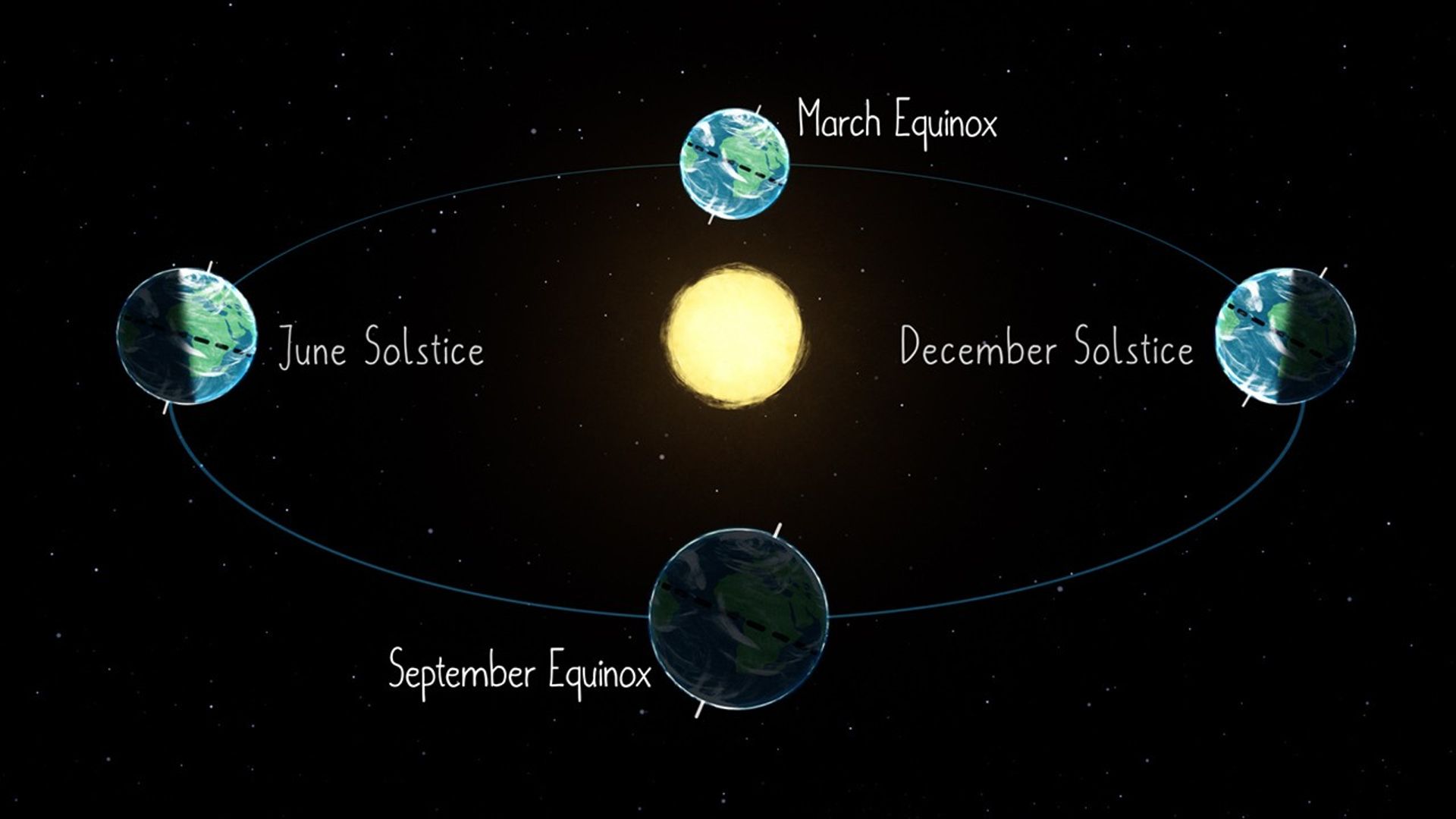
Illustration showing how Earth’s tilt leads to the Northern and Southern Hemispheres receiving changing amounts of sunlight over the course of the year. At the equinoxes, neither hemisphere is more tilted toward the Sun, so both hemispheres receive the same amount of sunlight.

Credits:
NASA/JPL-Caltech

Depending on your locale, equinoxes can be seen as harbingers of longer nights and gloomy weather, or promising beacons of nicer temperatures and more sunlight. Observing and predicting equinoxes is one of the earliest skills in humanity’s astronomical toolkit. Many ancient observatories around the world observed equinoxes along with the more pronounced solstices. These days, you don’t need your own observatory to know when an equinox occurs, since you’ll see it marked on your calendar twice a year! The word “equinox” originates from Latin, and translates to equal (equi-) night (-nox). But what exactly is an equinox?

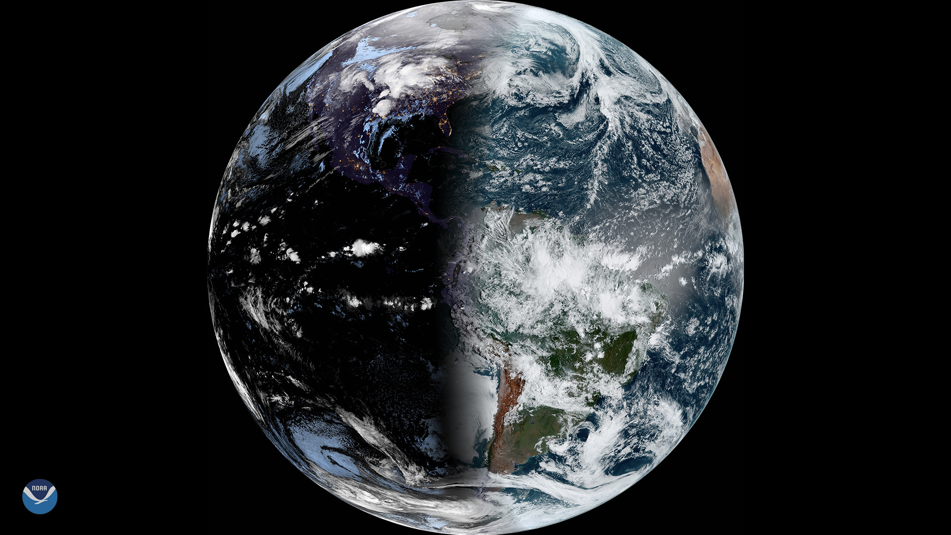
An equinox occurs twice every year, in March and September. In 2026, the equinoxes will occur on March 20, at exactly 14:46 UTC (or 7:46 AM EDT), and again on September 23, at 00:05 UTC (or September 22, 2026, at 5:05 PM PDT). The equinox marks the exact moment when the center of the Sun crosses the plane of our planet’s equator. The day of an equinox, observers at the equator will see the Sun directly overhead at noon. After the March equinox, observers anywhere on Earth will see the Sun’s path in the sky continue its movement further north every day until the June solstice, after which it begins traveling south. The Sun crosses the equatorial plane again during the September equinox, and continues traveling south until the December solstice, when it heads back north once again. This movement is why some refer to the March equinox as the northward equinox and the September equinox as the southward equinox.

A full disk view of the earth from GOES 16, GOES East on the vernal Equinox.
NOAA/NASA

Our Sun shines equally on both the Northern and Southern Hemispheres during equinoxes, which is why they are the only times of the year when the Earth’s North and South Poles are simultaneously lit by sunlight. Notably, the length of day and night on the equinox isn’t precisely equal; the date for that split depends on your latitude, and may occur a few days earlier or later than the equinox itself. The complicating factors? Our Sun and atmosphere! The Sun itself is a sphere and not a point light source, so its edge is refracted by our atmosphere as it rises and sets, which adds several minutes of light to every day. The Sun doesn’t neatly wink on and off at sunrise and sunset like a light bulb, and so there isn’t a perfect split of day and night on the equinox – but it’s very close.

Equinoxes are associated with the changing seasons. In March, Northern Hemisphere observers welcome the longer, warmer days heralded by their vernal, or spring, equinox, but Southern Hemisphere observers note the shorter days – and longer, cooler nights – signaled by their autumnal, or fall, equinox. Come September, the reverse is true.

Originally posted by Dave Prosper: February 2022

Last Updated by Kat Troche: March 2026

Source: science.nasa.gov
NASA-Funded Research Finds Complex Life Defying Record Heat

6 min read

NASA-Funded Research Finds Complex Life Defying Record Heat

This video shows Incendiamoeba cascadensis motility at 60ºC. When pushed to its limits in the lab, I. cascadensis can remain partially active at 150.8 degrees Fahrenheit (66 degrees Celsius) and can recover from exposure to a staggering 158 degrees Fahrenheit (70 degrees Celsius) for five minutes. However, 80 degrees Fahrenheit (176 degrees Celsius) proved to be too much for the amoeba to come back from.
Beryl Rappaport

NASA-supported scientists have discovered an organism that lives at extreme temperatures previously thought impossible for complex life. High temperatures can cause the destruction of necessary cell components, which is a big problem for cells with complex parts like a nucleus encasing delicate genetic information.

In the heated waters of California’s Lassen Volcanic National Park, a team of scientists observed an amoeba that can reproduce by division at an astonishing 145 degrees Fahrenheit (63 degree Celsius), setting a record for the upper temperature limit for all known eukaryotes. Incendiamoeba cascadensis, also dubbed the fire amoeba, stops reproducing above 145 degrees Fahrenheit but is still active, moving around to search for food at up to 147 degrees Fahrenheit (64 Celsius). The previous limit of 140 degrees Fahrenheit (60 Celsius) for eukaryotes was set by a few species of fungi and red algae. The results were published on Tuesday in the journal Cell.

Astrobiologists have long studied the boundaries of life’s survival on Earth to determine how organisms might live on other worlds like Mars where conditions are less hospitable than our home planet. Organisms that endure at the edges of habitability under extreme temperature, pH levels, radiation, and other environmental conditions are known as extremophiles. Studying them helps scientists understand what life as we know it is capable of. Extremophiles also produce unique proteins that can have promising uses in biotechnology, from industrial applications to medicine.

Previous extremophile research has mostly focused on single-celled bacteria and archaea. The new study shows that the more complex cells of eukaryotes might be more durable than previously thought and could even help scientists understand locations in the universe where complex life could survive.

Complex life on Earth

Life on Earth is broadly divided into two categories, prokaryotes and eukaryotes. Prokaryotes are single-cell organisms that do not have a nucleus or membrane-bound organelles inside their single cell. This means that they have less cellular ‘machinery’ that can be damaged by extremes, such as blistering heat, bitter cold, caustic acidity, or damaging radiation.

Organisms that live in extreme heat are known as thermophiles. To be a true ‘heat-loving’ thermophile, the organism must be able to replicate, move, eat, and survive above 113 degrees Fahrenheit (45 degrees Celsius).

Prokaryotes include bacteria and archaea, with archaea being particularly adept at surviving extremes. Because of their relative simplicity, scientists also believe that prokaryotes were the first forms of life to appear on Earth, billions of years ago when the environment of our planet was much more inhospitable than it is today.

Eukaryotes are more complicated organisms that are thought to have evolved later in the history of life on Earth. These organisms have a separate cell nucleus inside their cells that contains fragile genetic information. Eukaryotes also contain membrane-bound organelles, such as mitochondria and endoplasmic reticulum. These organelles are like mini cellular machines that perform specific functions. Eukaryotes include a wide span of life, from single-celled algae to multicellular organisms like plants and human beings.

Complexity in Extreme Heat

High temperatures lead to the breakdown of proteins and other biomolecules that living cells need to function. Heat also can cause membranes to break apart, thereby destroying cells. It has been suggested that organelle membranes in eukaryotes could not remain stable above 144 degrees Fahrenheit (62 degrees Celsius). The discovery of I. cascadensis proves that assumption wrong.

“In part, studies on eukaryotes may have been limited because of assumptions about membrane stability,” says Beryl Rappaport, graduate student at Syracuse University and lead author of the study. “We are hoping that the discovery of I. cascadensis encourages others to keep searching for high temperature eukaryotes.”

The team sequenced the I. cascadensis genome, studying the expression of genes at multiple temperatures. They found many genes that help the amoeba stabilize DNA and protect it from breaking down. Other genes allow the organisms to sense the external environment. At high temperatures, the expression of certain genes also increased, including those involved in maintaining protein folding.

“We were able to uncover many strategies that could help I. cascadensis survive at high temperatures, and some of these strategies could be used by thermophiles across all life,” says Rappaport. “For instance, some proteins in I. cascadensis have a high positive surface charge that could help them remain stable. These protein charges are similar to those found in thermophilic bacteria and archaea.”

The team also compared genetic information from other studies world-wide. In this trove of data, they found similar pieces of DNA from geothermal samples in places like New Zealand and Yellowstone National Park. This means that additional thermophilic amoebas related to I. cascadensis might be living all around the globe just waiting to be discovered.

The image shows an over the shoulder view of a scientist wearing a long sleeve blue shirt and a brown bucket hat for protection from the bright sun. They also have a high visibility vest on. They are reaching a sampling stick out toward a small stream of thermal water surrounded by tall grass. The water has brown/green slime around the edges.
Lead author Beryl Rappaport collecting samples of Incendiamoeba cascadensis in California’s Lassen Volcanic National Park. The organism’s name means “Fire amoeba coming from the cascades.” California’s Lassen Volcanic National Park is the southernmost active volcanic region in the Cascade Range and includes Lassen Peak, the world’s largest plug dome volcano.
Kristen Skruber

Search for life beyond Earth

Earth is the only planet we know of that is inhabited with life. For life as we know it to survive on other planets in the solar system or beyond, organisms might have to cope with environmental conditions that are very different from those found here at home.

“Studying extremophiles helps us better understand the biochemical and physiological limitations of life as we know it on Earth,” says Alison Olcott, program scientist for Exobiology at NASA Headquarters in Washington. “This information, in turn, helps guide NASA’s search for life as it expands the range of conditions we think life could potentially be inhabiting elsewhere.”

In particular, the study increases our understanding of where and how life with complex cells might persist on Earth and beyond.

“Finding eukaryotes surviving in high temperature environments not only expands our understanding of where life could be found, but also of how complex that life could be,” says Olcott.

However, the researchers do point out that survival depends on many factors that are part of a larger ecosystem.

“It could certainly be possible for complex life like I. cascadensis to survive on another planet, but Earth is the only planet we currently know of to have all the requirements for I. cascadensis to be happy,” says Rappaport. “It’s not just about temperature. An environment also needs the right acidity, oxygen levels, pressure, water, and food. I. cascadensis could not survive on its own. It needs other life to be supported as well.”

For more information on astrobiology at NASA, visit:

https://science.nasa.gov/astrobiology

Details

Last Updated

Sep 22, 2026

Source: science.nasa.gov

Risks of Decompression Sickness and Venous Thromboembolism during Spaceflight and Patent Foramen Ovale Implications

3 min read

Preparations for Next Moonwalk Simulations Underway (and Underwater)

PFO DCS VTE Working Group Photo September 2026
Top Row (from left to right): Michael Stenger, Joe Dervay, Steve Piper, Dave Francisco, Craig Kutz, Matthew Makowski, Alex Garbino, Hiroki Bochimoto, Doug Ebert, James Locke, Raffi Kuyumjian. Bottom Row (from left to right): Mark Crowther, Stephan Moll, Doug Ebersole, Mike Gernhardt, David Southerland, Sarah Taoufik
NASA

The purpose of this working group was to assemble a panel of experts to review the most recent data related to extravehicular activity (EVA) prebreathe testing and decompression sickness (DCS) events, venous thromboembolism (VTE) in-flight occurrences, and patent foramen ovale (PFO) implication as they relate to NASA’s Artemis (lunar and beyond) missions. The recommendations from this working group are built upon and integrate the outcomes of the September 2024 Assessment of Patent Foramen Ovale (PFO) as Related to Decompression Sickness (DCS) in the Spaceflight Environment and During Ground Testing (NASA/SP-20240010473), the April 2026 NASA Risk of Venous Thromboembolism in Spaceflight Working Group (NASA/SP- 20260005258/REV1), and the updated DCS prevention standard reviewed by the DCS panel in NASA-STD-3001 Volume 2 Human Factors, Habitability, and Environmental Health (NASA-STD-3001 Vol 2 Rev F), with a specific focus on risk mitigation interventions such as PFO closure.

Recommendations

The following is a summary of the working group’s recommendations:

  1. Ground-based studies should no longer remove subjects from research solely due to the presence of LVGE. Protocols should balance subject safety with population representativeness, and subjects must be fully informed of their LVGE status and any associated risks.
  2. The consensus was that the presence of a PFO is not considered a major risk factor for VTE formation, nor for complications from an embolism traveling from an initial formation site in the left internal jugular or cerebrum at normoxic or proposed hypoxic space habitats. No changes to astronaut selection criteria regarding PFOs are recommended with respect to VTE.
  3. The consensus of the group is that there is no definitive link between bubble grades and the risk of DCS at altitude for prebreathe protocols involving partial gravity and ambulation.
  4. The panel concluded that while minimizing bubbles is desirable, the predictive value of bubble scores for DCS remains uncertain, especially for lunar surface operations.
  5. It was determined that a “small” PFO (Grade 1 or 2) does not pose a significant risk. There were mixed opinions on whether closing or screening out crew members with a “large” PFO (Grade 3 or above) significantly reduces the risk of a venous gas embolism (VGE) passing to the arterial side and causing a significant mission health event. The group did not recommend universal screening or exclusion of astronauts with large PFOs but emphasized the importance of risk mitigation through protocol design and ongoing data collection. If crews are assessed, they should be informed of their status and offered closure for a large PFO.
  6. The panel concluded that clear clinical guidance is required regarding medication use for all crewmembers prior to Extravehicular Activities (EVAs). Specifically, protocols must address the use of aspirin for Decompression Sickness (DCS) prevention and pain relief. Additionally, guidance is needed for the pre and post-EVA use of analgesics (acetaminophen, ibuprofen, naproxen, celecoxib), as these medications have the potential to mask DCS symptoms.

Source: www.nasa.gov